Best MATLAB Gradient Calculation Tools to Buy in April 2026

Learning to Program with MATLAB: Building GUI Tools


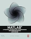
MATLAB: A Practical Introduction to Programming and Problem Solving


Learning to Program with MATLAB: Building GUI Tools


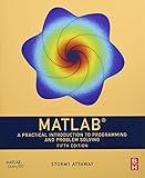
MATLAB: A Practical Introduction to Programming and Problem Solving


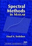
Spectral Methods in MATLAB (Software, Environments, Tools)
- AFFORDABLE PRICE: ENJOY SIGNIFICANT SAVINGS ON QUALITY READING MATERIAL.
- SUSTAINABLE CHOICE: SUPPORT RECYCLING BY BUYING PRE-LOVED BOOKS.
- QUALITY ASSURANCE: CAREFULLY INSPECTED FOR GOOD CONDITION AND READABILITY.


Antenna and EM Modeling with MATLAB Antenna Toolbox


MATLAB Symbolic Algebra and Calculus Tools


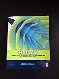
Matlab: A Practical Introduction to Programming and Problem Solving


MATLAB Fundamentals for Mechanical Engineers


To calculate the gradient in MATLAB, you can use the "gradient" function. This function calculates the numerical gradient of a scalar function across an array. The syntax for using the "gradient" function is as follows:
[dx, dy, dz, ...] = gradient(f, spacing)
Here, "f" represents the input scalar function, and "spacing" denotes the sample spacing in each dimension. The "gradient" function returns the gradients in each dimension, such as "dx" for the gradient in the x-direction, "dy" for the gradient in the y-direction, and so on.
For example, consider the following code that calculates and visualizes the gradient of a 2D scalar function:
% Define the scalar function [X, Y] = meshgrid(-5:0.1:5, -5:0.1:5); Z = sin(X) + cos(Y);
% Calculate the gradient [dZdx, dZdy] = gradient(Z, 0.1);
% Plot the scalar function and its gradient vectors figure; surf(X, Y, Z); hold on; quiver(X, Y, dZdx, dZdy, 'r'); xlabel('X'); ylabel('Y'); zlabel('Z'); title('Scalar Function with Gradient Vectors');
In this example, we first define a scalar function "Z" using the "meshgrid" function. Then, we use the "gradient" function to calculate the gradients "dZdx" and "dZdy" with a sample spacing of 0.1. Finally, we plot the scalar function using the "surf" function and overlay the gradient vectors using the "quiver" function.
By utilizing the "gradient" function, you can easily calculate and analyze the gradients of scalar functions in MATLAB for different applications.
What is the concept of neighborhood pixels in gradient computation?
In gradient computation, the concept of neighborhood pixels refers to the idea of considering the surrounding pixels of a particular pixel when calculating the gradient or the rate of change of intensity.
When calculating the gradient, the pixels in the neighborhood are analyzed to determine the variations in intensity or color values. This information is used to estimate the direction and magnitude of the gradient at that pixel.
Different methods or algorithms can define the specific size and shape of the neighborhood around a pixel. For example, a common approach is to consider a 3x3 or 5x5 square neighborhood, where the pixel of interest is at the center. The intensity values for these neighboring pixels are then used to calculate the gradient.
By considering the neighborhood pixels, the gradient computation can capture more local image variations, providing more detailed information about the changes in intensity or color across the image. This information is useful in various image processing tasks, such as edge detection, image enhancement, and feature extraction.
What is the purpose of calculating the gradient in MATLAB?
The purpose of calculating the gradient in MATLAB is to compute the rate of change of a function with respect to its input variables. The gradient is a vector that consists of partial derivatives of a function, which indicates both the direction and magnitude of the steepest ascent or descent in that function.
By calculating the gradient, MATLAB allows for optimization and numerical analysis techniques that utilize this information to find local or global extrema of a function. It is commonly used in solving problems related to machine learning, optimization, signal processing, and many other disciplines where optimization and analysis of functions are required.
How to implement gradient-based image segmentation in MATLAB?
To implement gradient-based image segmentation in MATLAB, you can follow these steps:
- Read the input image using the imread function and convert it to grayscale using the rgb2gray function if needed.
- Preprocess the image if necessary. This may include smoothing or denoising to improve the quality of the gradient calculation.
- Compute the gradient magnitude image using the imgradient or imgradientxy function. These functions calculate the gradient magnitude or both gradient magnitude and direction.
- Threshold the gradient magnitude image to create a binary edge map. The threshold value can be determined manually or automatically using techniques such as Otsu's method or edge intensity analysis.
- Optionally, you can perform morphological operations such as dilation or erosion on the binary edge map to refine the segmentation result.
- Apply a region growing algorithm or graph cut algorithm to group the pixels based on the gradient information. This step will generate the segmented regions.
- Visualize the segmentation result using the imshow function or save it to the disk using the imwrite function.
Here is an example code snippet demonstrating gradient-based image segmentation using the steps mentioned above:
% Step 1: Read the input image image = imread('input_image.jpg'); gray_image = rgb2gray(image);
% Step 2: Preprocess the image if needed
% Step 3: Compute the gradient magnitude image [gradient_magnitude, gradient_direction] = imgradientxy(gray_image);
% Step 4: Threshold the gradient magnitude image threshold = graythresh(gradient_magnitude); binary_edge_map = imbinarize(gradient_magnitude, threshold);
% Step 5: Morphological operations (optional)
% Step 6: Apply region growing or graph cut algorithm
% Step 7: Visualize or save the segmentation result imshow(binary_edge_map);
Note that this is a basic implementation, and more advanced techniques can be applied to improve the segmentation accuracy or handle specific cases.
